Some nonlinear learning

Clustering, and our favorite: sparse coding

Foldiak 1990.

Last post, we talked about the limits of representation learning in linear neuron models. In PCA, implemented by Sanger’s rule, we only consider pairwise correlations of inputs.

What happens if we want to look at higher-order correlations? A logical next step is nonlinear Hebbian learning. Suppose we now have a neuron with some nonlinear function f. i indexes the inputs x and corresponding weights w.

\(y=f(\sum_i w_i x_i)\)

Our Hebbian update rule becomes

\(\begin{aligned} \Delta w_{i} &\propto y_ix_i \\ &= f(\sum_jw_{j}x_j)x_i \\ &= k_0x_i + k_1 \sum_j w_j x_i + k_2\sum_{jk} w_j w_k x_kx_j x_i + ... \end{aligned}\)

where j indexes all the neurons in the network. If you do a Taylor expansion, your weight updates are now a function of three- and higher-point correlations between units x_i, x_j, x_k… But what you get exactly of course depends on f.

Winner-take-all

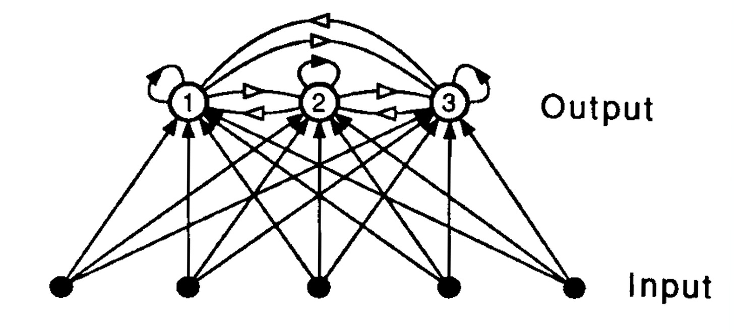
How do we pick f? This depends on the structure of the data. Suppose our data come from discrete groups, or clusters, where we do not have ground truth labels for each point. For example, an animal identifying an odorant from olfactory input. Our network looks like this, where black arrows are excitation, and white arrows are inhibition.

We can take f to be the winner-take-all function. That is, y_i is 1 if the input has the highest inner product with the ith weight compared to other weights, and 0 otherwise.

\( y_i = \begin{cases} 1 & \sum_k w_{ik}x_k > \sum_k w_{jk} x_k\, \, \forall i \neq j \\ 0 & \text{otherwise} \end{cases}\)

E.g. for output unit ① to turn on, the inner product of its weights and the input would have to be higher than the every other unit’s weights’ inner product with the input. The learning rule is

\(\Delta w_{ij} = \eta y_i (x_j - w_{ij})\)

which says that the cluster center moves toward the points that were assigned to it.

This results in a discrete clustering algorithm: given a dataset, assign each point to a cluster that contains other points similar to it. This is also a form of competitive learning, as seen literally in the winner-take-all function, meaning that neurons have the ability to turn other neurons off in the appropriate situation.

x are cluster centers (randomly initialized), and • are data points. After learning cluster centers (weights) from the points, each point is assigned to a cluster.

In an abstract neural circuit, you could think of winner-take-all as 1-sparse network: given some input, exactly one neuron fires in response. But there are obvious limitations to the winner-take-all algorithm. What if we can’t assume that each input corresponds to exactly what one neuron is coding? What if activity is distributed across a population of neurons?

Sparse coding

Suppose we could assign multiple clusters to each data point. We could use these assignments (AKA weights) to linearly combine different clusters to describe each data point. Said another way: rather than representing one concept with one neuron, we could represent one concept using a small set of neurons, where the rest of the neurons are silent. This is sparse coding.

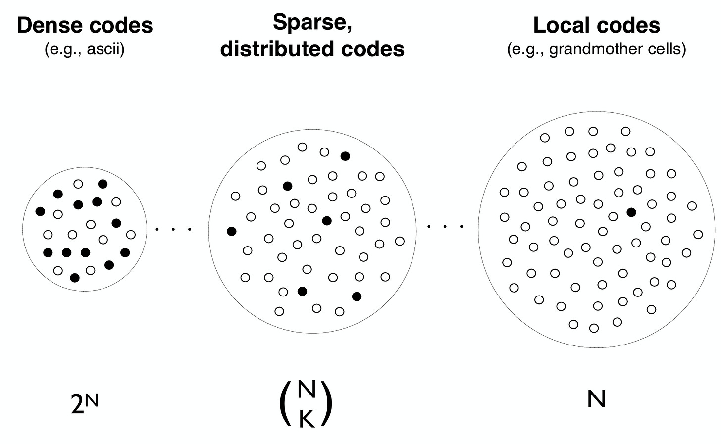
In the below figure, we show a range of coding schemes, each with its own pros and cons. In a dense binary code, you can represent 2^N concepts where N is the number of neurons, but it is brittle: changing one unit can completely change the output. Plus, more neurons will be firing at once, which is less energy efficient, and it is nontrivial to decode information from the neural activity. On the other end of the spectrum, local codes are winner-take-all AKA a lookup table AKA “grandmother cells”¹: for each concept, exactly one neuron fires. You can only represent up to N concepts, and if one neuron is destroyed, you can no longer represent the corresponding concept. But it requires very little energy, and can be decoded easily by a direct readout.

A sparse code is then somewhere in the middle: it is more robust to noise and perturbations, and can represent up to N choose K patterns, where K « N is the number of active neurons.

Each type of representation (here all binary) has its pros and cons.

In his quest to relate sensory perception to neural activity, Horace Barlow proposed the concept of sparse coding in 1972 as one of five dogmas:

2. The sensory system is organized to achieve as complete a representation of the sensory stimulus as possible with the minimum number of active neurons.

Peter Földiák first created a neural learning algorithm for sparse coding in 1990. Bruno Olshausen & David Field showed in 1996 that maximizing image reconstruction and sparsity of neural activity results in learning localized, oriented, and bandpass features that resemble receptive fields in mammalian primary visual cortex².

A subset of features learned from sparse coding on natural images.

Why do these features look the way they do? Learning them can be thought of abstractly as an evolutionary process to develop optimal representations (i.e. receptive fields). They are adapted to the low-level statistics of natural scenes, which contain localized oriented edges³, and learning oriented features requires seeing correlations beyond pairwise⁴. Sparse coding provides a way to do this.

Mathematically, the goal of sparse coding is learn the features Φ and infer the neural activity a that minimize the energy function E:

\(E = \lVert x - \Phi a \rVert_2^2 + \lambda \lVert a \rVert_1\)

Where x is the input image, and λ is a scalar that controls the strength of the sparsity penalty. The first term encourages reconstruction of the image, and the second encourages sparsity of the coefficients. Note that this is a generative model: we reconstruct the image using a linear combination of features

\(x = \Phi a + \epsilon\)

where ϵ is some random measurement or image noise.

Inferring the activity amounts to producing the sparsest coefficients that best reconstruct the image using the given features⁵. Unlike in standard machine learning, we use inference here to mean an iterative procedure that outputs relevant factors a given input data⁶. Although the generative model is linear, inference itself is recurrent and nonlinear: updating the activity of one neuron depends on the activity of all the neurons in the previous time step. Because of the sparsity constraint, this can also be thought of as competitive learning⁷.

Sparse coding is an unsupervised feature learning algorithm that has lots of advantages to previous methods we discussed. Outside of vision, there has been experimental evidence for sparse coding in other systems in other animals (see Olshausen & Field 2004 for a review). But there are of course limitations. A clear one is the inability of a sparse code to capture spatial transformations, or more abstract similarities. The next post will focus on one method that starts to address this: manifold learning.

1. This term comes from the idea that there is a cell that fires when you see your grandmother. There has been experimental evidence for this in a guy who had a Jennifer Aniston cell, though apparently he was also just obsessed with Jennifer Anniston, so… 🤷🏻‍♀️

2. I wrote a simple sparse coding tutorial here.

3. Unfortunately I don’t have time to go into this here, but much of the motivation for sparse coding from natural scene statistics comes from Field 1994.

4. For example, PCA on natural images (considering only pairwise correlations) results in non-localized and generally non-oriented features.

5. Given a set of features, there are many ways to infer coefficients: standard gradient descent, the more neurally-plausible locally competitive algorithm, ISTA/FISTA, etc.

6. Bruno’s book chapter on perception as inference.

7. The concept of explaining away is very important in sparse coding inference, and separates it from feedforward filtering algorithms that also produce activity given a set of features. On the left, we see two receptive fields representing two cells, overlaid on an edge. For feedforward neurons (the output is just the inner product between the receptive field and the pixels underneath), the tilted cell would have only a slightly lower firing rate than the upright one, because both receptive fields match decently well with the edge orientation and polarity. However, in sparse coding, the tiled cell would be suppressed by the upright cell, because the upright cell is better aligned with the edge. This suppression also results in a sparser representation.

Competitive learning and explaining away can be better explained through LCA.